

Plotting post hoc tests with Python
combining scikit-posthocs with statannotations
When three or more groups of samples are compared (e.g. Using ANOVA/Tukey HSD or Kruskal-Wallis/Dunn), you’ll often see results shown as a boxplot, with lines highlighting which groups are significantly different. In Python there is no single package to do this quickly, though by combining scikit-posthocs with statannotations similar plots can be generated with relative ease. Here we’ll go over the code involved step by step.

Statistical tests comparing three or more groups are typically done in two steps. The first test will check if there are any statistical difference between the groups, the second test will then tell you which groups are different. The second test is referred to as a post hoc test. While there are many combinations of tests to choose from, common combinations are Kruskal-Wallis followed by a post hoc Dunn’s test (non-parametric) and ANOVA with Tukey’s Honest Significant Differences (parametric). Though note that the code below can easily be adapted for other tests.
All code from this post can be found on GitHub and Binder.
The data
The iris dataset, with measurements of petal and sepals of three species of flowers will be a nice way to test some of these test. The code below will load all required libraries and load the iris data which is included in scikit-learn.
%load_ext nb_black
from sklearn.datasets import load_iris
import pandas as pd
import seaborn as sns
import matplotlib.pyplot as plt
import numpy as np

iris_obj = load_iris()
iris_df = pd.DataFrame(iris_obj.data, columns=iris_obj.feature_names)

iris_df["species"] = [iris_obj.target_names[s] for s in iris_obj.target]
iris_df.head()
| sepal length (cm) | sepal width (cm) | petal length (cm) | petal width (cm) | species | |
|---|---|---|---|---|---|
| 0 | 5.1 | 3.5 | 1.4 | 0.2 | setosa |
| 1 | 4.9 | 3.0 | 1.4 | 0.2 | setosa |
| 2 | 4.7 | 3.2 | 1.3 | 0.2 | setosa |
| 3 | 4.6 | 3.1 | 1.5 | 0.2 | setosa |
| 4 | 5.0 | 3.6 | 1.4 | 0.2 | setosa |
For the first test (Kruskal-Wallis and ANOVA) we’ll use the implementations from SciPy and these require for each group a list of values to be passed as a function parameter. The easiest way to do so is with the code below, a list of lists is created with for each species the sepal lengths. This can then be unpacked to parameters using the asterisk (*).
species = np.unique(iris_df.species)

data = []

for s in species:
    data.append(iris_df[iris_df.species == s]["sepal length (cm)"])
Kruskal-Wallis with Dunn’s
The Kruskal-Wallis test is included in SciPy and can easily be applied to our data after it was properly structured in the previous step.
from scipy import stats

stats.kruskal(*data)
This will return a statistic (96.04) and a p-value (8.9e-22) so there is a significant difference between these species.
However, this test will not show us between which species there are difference. To know this we need to apply a post hoc
Dunn’s test, often used in combination with Kruskal-Wallis. The posthoc_dunn()function included in
scikit-posthocs can be used. (Note the difference in syntax with SciPy’s test)
from scikit_posthocs import posthoc_dunn

# posthoc dunn test, with correction for multiple testing
dunn_df = posthoc_dunn(
    iris_df, val_col="sepal length (cm)", group_col="species", p_adjust="fdr_bh"
)
dunn_df
This will return a matrix with all pairwise combinations of species and the p-value of the test (with correction
applied if p_adjust is set to a valid method).
| setosa | versicolor | virginica | |
|---|---|---|---|
| setosa | 1.000000e+00 | 1.529257e-09 | 6.000296e-22 |
| versicolor | 1.529257e-09 | 1.000000e+00 | 2.774866e-04 |
| virginica | 6.000296e-22 | 2.774866e-04 | 1.000000e+00 |
So in this case each species is significantly different from the other two. We’ll have a look at ANOVA and Tukey HSD first before going into details how to visualize these results better.
ANOVA with Tukey HSD
Similarly to the previous example, we can run an ANOVA. First we run the f_oneway(), which is the function in
SciPy to do an ANOVA, and finish with posthoc_tukey() from scikit-posthocs.
The first test gives us a significant p-value (1.67e-31), so it is good to continue with the Tukey test.
from scikit_posthocs import posthoc_tukey

# First we do a oneway ANOVA as implemented in SciPy
print(stats.f_oneway(*data))

tukey_df = posthoc_tukey(iris_df, val_col="sepal length (cm)", group_col="species")
tukey_df
This gives us the finale table with all comparisons and p-values from those tests.
| setosa | versicolor | virginica | |
|---|---|---|---|
| setosa | 1.000 | 0.001 | 0.001 |
| versicolor | 0.001 | 1.000 | 0.001 |
| virginica | 0.001 | 0.001 | 1.000 |
Visualizing the results
These matrices are hard to interpret, and most will prefer a simple visualization to highlight significant differences. While showing the actual data using seaborn is easy, adding in annotated lines with the p-values isn’t. This is where statannotations comes in, this package allows you to add those in with a few lines of code. While the package comes with its own suite of statistical tests, post hoc tests unfortunately aren’t currently included. So here is how to do this.
First, the matrix needs to be converted to a non-redundant list of comparisons with the p-value. This is done by
removing the lower half and diagonal of the matrix and turning the matrix format into a long dataframe using
melt(). The code and resulting dataframe are shown below.
remove = np.tril(np.ones(tukey_df.shape), k=0).astype("bool")
tukey_df[remove] = np.nan

molten_df = tukey_df.melt(ignore_index=False).reset_index().dropna()
molten_df
| index | variable | value | |
|---|---|---|---|
| 3 | setosa | versicolor | 0.001 |
| 6 | setosa | virginica | 0.001 |
| 7 | versicolor | virginica | 0.001 |
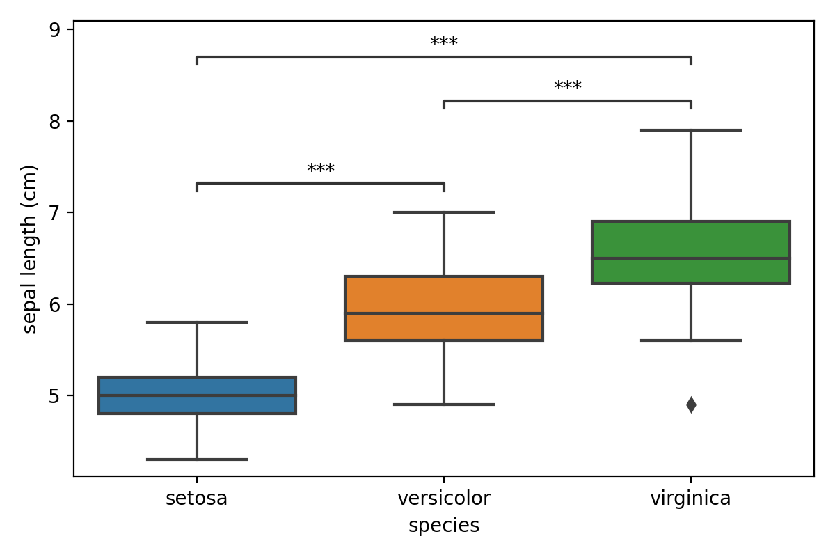
Next, we’ll have to draw the main plot using seaborn’s boxplot() function and convert our dataframe into
a list of pairs and list of matching p-values for statannotations. The code below is a little cryptic due to the use
of list comprehensions and iterrows(), though in a nutshell it will go over each row and create a tuple with the
species that are being compared. Then p-values are converted to a list using the same functions.
The list of pairs is passed to an Annotator object along with the data. By calling
configure() the plot is set up as we would like. Finally p-values are added using set_pvalues_and_annotate()
which will also add the annotations to the plot.
import seaborn as sns
from statannotations.Annotator import Annotator

ax = sns.boxplot(data=iris_df, x="species", y="sepal length (cm)", order=species)

pairs = [(i[1]["index"], i[1]["variable"]) for i in molten_df.iterrows()]
p_values = [i[1]["value"] for i in molten_df.iterrows()]

annotator = Annotator(
    ax, pairs, data=iris_df, x="species", y="sepal length (cm)", order=species
)
annotator.configure(text_format="star", loc="inside")
annotator.set_pvalues_and_annotate(p_values)

plt.tight_layout()
Conclusion
While it is a shame there is no package out (yet) that makes these stats and visualization a one-liner (like the R package ggpubr), with these bits of code it is easy enough to do this ourselves.
Liked this post ? You can buy me a coffee