
Clustering the Palmer Station penguin data, using PyMC3
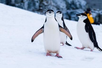
Adelie, Chinstrap, Gentoo...
This post will be all about trying to infer the species various observations originated from, without actually having access to the labels. This might sound like a far-fetched example, but it happens more often than you might expect in biology! When studying large animals you can usually find clear differences between species, but when studying nematodes (tiny worms) in a soil sample those differences might be very hard to spot! You can also have a sub-population that slightly differs from the main community, for instance polyploid plants (with extra copies of their genome) might grow in the same field as plants with normal ploidy. These are considered the same species and are similar in most ways, except a bit bigger or stronger or more tolerant, so while making initial measurements these might not stand out. Or indirect measurements, some animals are rare and live in remote places, so biologists might use footprints to study those animals. If multiple species leave similar prints … they might have to resort to using their size, distance between them, … to estimate which exact species a set of prints belongs to. So the solution is to measure as many subjects as possible and (hopefully) figure it out later on.
It is particularly challenging to identify different groups if you don’t know even know how many groups there are. Here the Palmer Station Penguin dataset is used, to show the issue (we’ll hide the species labels from the models), and we’ll try to identify how many species there are in the set, and which subjects belong to the same group using flipper, bill and body mass measurements from each subject.
Notebooks with the data and full code for this post can be found in this GitHub repo. There you’ll also find the code applied to other datasets like the Iris and Fish Market datasets (albeit with less documentation).
Loading the data
The GitHub repo contains the data in a .csv format that can be loaded directly using pandas. We don’t need the
island where the observation was made or the sex of the animal, so these columns are dropped. Rows with remaining
missing values are omitted using .dropna(). We do keep the species label, so later on we can check if
our clustering is actually working, but it will not be used during the clustering.
%load_ext nb_black
import seaborn as sns
import pymc3 as pm
import pandas as pd
import numpy as np
import arviz as az

import altair as alt

penguin_df = (
    pd.read_csv("./data/penguins_size.csv").drop(columns=["island", "sex"]).dropna()
)
penguin_df
The data is best scaled, so the mean of each feature will be zero with a standard deviation of one. StandardScaler
makes this easy.
from sklearn.preprocessing import StandardScaler

scaler = StandardScaler()
scaled_penguin_df = scaler.fit_transform(penguin_df.drop(columns=["species"]))
scaled_penguin_df = pd.DataFrame(scaled_penguin_df, columns=penguin_df.columns[1:])
scaled_penguin_df["species"] = list(penguin_df["species"])
scaled_penguin_df
The first model - using a single feature
All models in this post have a pm.Dirichlet distribution at their core which defines the probabilities of observing
a certain group, in this case species. For now, we’ll define the number of clusters we want using n_clusters,
we’ll work around this later, don’t worry! Next, we assign categories to all observations based on those probabilities.
Explicitly including categories using pm.Categorical makes is really straightforward to extract groups later, note
however that there are more efficient ways using pm.NormalMixture if we would just be interested in fitting a
model.
Here we include a sigma and a mean for each category, and create a likelihood function using those to fit a normal distribution on the body mass observations of each species.
n_clusters = 3
n_observations, n_features = scaled_penguin_df.shape

with pm.Model() as model:
    p = pm.Dirichlet("p", a=np.ones(n_clusters))
    category = pm.Categorical("category", p=p, shape=n_observations)

    bm_sigmas = pm.HalfNormal("bm_sigmas", sigma=1, shape=n_clusters)
    bm_means = pm.Normal("bm_means", np.zeros(n_clusters), sd=1, shape=n_clusters)

    y_bm = pm.Normal(
        "y_bm",
        mu=bm_means[category],
        sd=bm_sigmas[category],
        observed=scaled_penguin_df.body_mass_g,
    )

    trace = pm.sample(10000)
After sampling, we can pull out the categories from one of the traces and compare this to the actual species to see how well it worked. We’ll add the groups back to the original data, quickly reformat it to get counts, and visualize using Altair.
[2][200] points to the chain at index two and the trace at index 200, when doing this exercise inspect
multiple to get an impression of the overall performance.
groups = [
    f"Group {n+1}"
    for n in list(trace.get_values("category", burn=6000, combine=False)[2][20])
]
penguin_df["group"] = groups

plot_df = penguin_df.groupby(["species", "group"]).size().reset_index(name="counts")

alt.Chart(plot_df).mark_bar().encode(
    x=alt.X("group", title=None),
    y=alt.Y("counts", title="Count"),
    color=alt.Color("species", title="Species"),
    tooltip=["group", "counts", "species"],
).properties(width=400)
Here you can see that Group 2 contains all Gentoo penguins (these are the largest and heaviest), but adds in a few of the others. The other two groups contain a mix of Adelie and Chinstrap penguins, not particularly impressive as a classifier. Let’s have a look the data we provided to the model before proceeding.
As you can see, there is a ton of overlap between the species, not ideal for such a simple classifier to distinguish. So, we should include more measurements, like the flipper length and culmen (part of the beak) length and depth.
A model that includes all features
The easiest way to expand this model is by simply adding more sigmas, means and likelihoods to it all sharing the categories.
n_clusters = 3
n_observations, n_features = scaled_penguin_df.shape
with pm.Model() as model:
    p = pm.Dirichlet("p", a=np.ones(n_clusters))
    category = pm.Categorical("category", p=p, shape=n_observations)

    cl_sigmas = pm.HalfNormal("cl_sigmas", sigma=1, shape=n_clusters)
    cd_sigmas = pm.HalfNormal("cd_sigmas", sigma=1, shape=n_clusters)
    fl_sigmas = pm.HalfNormal("fl_sigmas", sigma=1, shape=n_clusters)
    bm_sigmas = pm.HalfNormal("bm_sigmas", sigma=1, shape=n_clusters)

    cl_means = pm.Normal("cl_means", np.zeros(n_clusters), sd=1, shape=n_clusters)
    cd_means = pm.Normal("cd_means", np.zeros(n_clusters), sd=1, shape=n_clusters)
    fl_means = pm.Normal("fl_means", np.zeros(n_clusters), sd=1, shape=n_clusters)
    bm_means = pm.Normal("bm_means", np.zeros(n_clusters), sd=1, shape=n_clusters)

    y_cl = pm.Normal(
        "y_cl",
        mu=cl_means[category],
        sd=cl_sigmas[category],
        observed=scaled_penguin_df.culmen_length_mm,
    )
    y_cd = pm.Normal(
        "y_cd",
        mu=cd_means[category],
        sd=cd_sigmas[category],
        observed=scaled_penguin_df.culmen_depth_mm,
    )
    y_fl = pm.Normal(
        "y_fl",
        mu=fl_means[category],
        sd=fl_sigmas[category],
        observed=scaled_penguin_df.flipper_length_mm,
    )
    y_bm = pm.Normal(
        "y_bm",
        mu=bm_means[category],
        sd=bm_sigmas[category],
        observed=scaled_penguin_df.body_mass_g,
    )

    trace = pm.sample(10000)
This certainly works, though this would benefit from a loop instead of repeating code for each feature. However, is it any better than the previous model. Let’s have a look at a randomly selected chain/trace.
This certainly is a much better classification, which is confirmed by looking at multiple traces. All Gentoos are huddled together in group one, group three contains mostly Adelies, though group two is a bit of a mixed batch.However, this model has a big downside, multiple likelihoods. This makes it very hard to use PyMC3 and Arviz to compare the model with other models. It is not impossible, and in the GitHub repo there is a notebook where some code is included to do this, but this was very convoluted and definitely something to avoid where possible.
Switching to multivariate normal distributions
So to solve the issue with multiple likelihoods, pm.MvNormal can be used, this is a multivariate normal or
gaussian distribution which takes multiple input values and combines them into a single likelihood. It requires a mean
for each feature in the input and a Cholesky decomposition of covariance matrix… Jikes, I won’t pretend I know the
underlying mathematics, I don’t, but fortunately I found a bit of code that generates the required
matrix using pm.LKJCholeskyCov. In a nutshell this is required to take correlations between different features
into account.
Apart from that, this makes the code considerably cleaner and more generic than the previous model, so that is a nice free little bonus too.
n_clusters = 3
data = scaled_penguin_df.drop(columns=["species"]).values
n_observations, n_features = data.shape
with pm.Model() as model:
    chol, corr, stds = pm.LKJCholeskyCov(
        "chol",
        n=n_features,
        eta=2.0,
        sd_dist=pm.Exponential.dist(1.0),
        compute_corr=True,
    )
    cov = pm.Deterministic("cov", chol.dot(chol.T))
    mu = pm.Normal(
        "mu", 0.0, 1.5, shape=(n_clusters, n_features), testval=data.mean(axis=0)
    )

    p = pm.Dirichlet("p", a=np.ones(n_clusters))
    category = pm.Categorical("category", p=p, shape=n_observations)

    y = pm.MvNormal("y", mu[category], chol=chol, observed=data)

    trace = pm.sample(8000)
As a multivariate gaussian looks at the likelihood of seeing combinations of features it is also a better suited method for these data. So we are rewarded with a better fitting model too, just look at the classification below, which is nearly perfect!
How to determine the number of clusters
So far we hard, coded the number of clusters we wanted. Which is nice if you know this, but if you have no clue … In this case you need to build a model with 2, 3, 4, 5 … clusters and see which one gives the best fit, without being to complex. We’ll first create a function that create a model with n clusters, samples this and returns the model and traces. Then we’ll run and store this with multiple cluster sizes and use Arviz to compare these.
def run_model(data, n_clusters, samples=4000):
    print(f"Building model with {n_clusters} cluster and {samples} samples.")

    n_observations, n_features = data.shape
    with pm.Model() as model:
        chol, corr, stds = pm.LKJCholeskyCov(
            "chol",
            n=n_features,
            eta=2.0,
            sd_dist=pm.Exponential.dist(1.0),
            compute_corr=True,
        )
        mu = pm.Normal(
            "mu", 0.0, 1.5, shape=(n_clusters, n_features), testval=data.mean(axis=0)
        )

        p = pm.Dirichlet("p", a=np.ones(n_clusters))
        category = pm.Categorical("category", p=p, shape=n_observations)

        y = pm.MvNormal("y", mu[category], chol=chol, observed=data)

        trace = pm.sample(samples)
    return model, trace
This is actually a very generic function that will accept any dataframe or matrix (it should be scaled though), and a
number of clusters, builds and samples a models which it then returns. With a few lines of code we can run this and
capture the output in a dictionary. Then we use az.compare to compare the models with different numbers of
clusters.
data = scaled_penguin_df.drop(columns=["species"]).values
model_traces = {
    f"model_{i}_clusters": run_model(data, i, samples=8000) for i in range(2, 6)
}
comp = az.compare({k: v[1] for k, v in model_traces.items()})
comp
| rank | loo | p_loo | d_loo | weight | se | dse | warning | loo_scale | |
|---|---|---|---|---|---|---|---|---|---|
| model_3_clusters | 0 | -905.740656 | 68.837020 | 0.000000 | 4.808971e-01 | 29.476505 | 0.000000 | True | log |
| model_5_clusters | 1 | -905.837578 | 197.606731 | 0.096921 | 5.191029e-01 | 28.926480 | 11.295538 | True | log |
| model_4_clusters | 2 | -922.262126 | 175.651671 | 16.521469 | 0.000000e+00 | 29.039549 | 10.030136 | True | log |
| model_2_clusters | 3 | -1284.311894 | 156.435489 | 378.571238 | 2.416753e-09 | 28.624421 | 16.756834 | True | log |
Using az.compare there are a number of metrics applied to see which model is the best fit to our data. This
uses by default Leave-one-out cross-validation, and loo, p_loo and d_loo are the numbers coming out of
that analysis (loo is the metric to check, lower is better, p_loo is the estimated number of parameters and d_loo is
the difference with the best model). The weight can roughly be seen as the probability the model is correct given the
data, here closer to 1 is better. The standard error on the cross-validation, se in the table, is also included
as well the difference with between the models with the best model, dse.
We can see that the model with three clusters actually performs the best here. As this isn’t the maximum number of
clusters tested we should accept this. However, often it is not that clear from these numbers which model should be
picked, two models might be very close, … So plotting this out using az.plot_compare can help us sort this out.
az.plot_compare(comp)
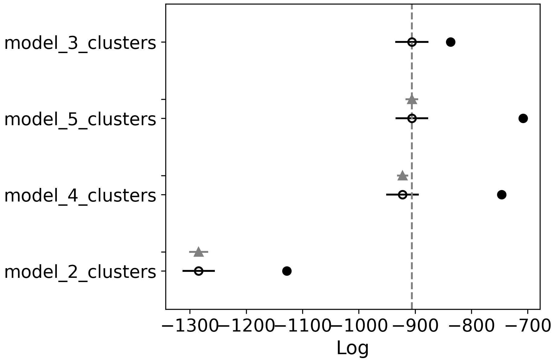
Here you can see the scores for all models, the vertical gray line marks the best score. Though you can probably consider all models where the black bar intersects with this line as equally good (in this case models with 3, 4 and 5 clusters). So in that case pick the one with the least clusters, even if it isn’t the top ranked one.
Conclusion
As I’ve only been working with PyMC3 and Bayesian Statistics for a month or two, some concepts here are beyond what I fully understand. Take everything here with a rather large pinch of salt! However, by going slow and taking one step at the time, it was still possible to build a very performant classifier for this dataset. It also gives me a push towards which theory to study up on (Multivariate Gaussians).
References
- palmerpenguins: Palmer Archipelago (Antarctica) penguin data. Allison Marie Horst and Alison Presmanes Hill and Kristen B Gorman (2020).
Acknowledgements
Header photo by Derek Oyen on Unsplash
Liked this post ? You can buy me a coffee