
Bayesian analysis of sales data, using PyMC3
Bayesian analysis and probabilistic programming is fairly different from ‘regular’ analysis. So here I’ll take you through my first attempt at using PyMC3 to analyse sales data of KeyForge decks and explore the effects of COVID-19 restrictions and releasing new content. PyMC3 takes some getting used to, but at the end you’ll see there are some clear advantages of this approach!
In this post we are looking at KeyForge sales, a collectible card game from FFG, which is in many ways unique. However, for sake of this post there are just a few things that matter; the game is sold as individual decks or starter kits with two decks (and some tokens to play the game). Each deck is randomly generated and unique, decks are supposed to be played as is, without changing the cards. Players are encouraged to scan a QR code included with each deck using the companion app to register it online. The number of decks that has been registered since KeyForge’s release in November 2018 can be found on their website. New sets are released every six to eight months with new cards and new mechanics, prior to each release there is a period where new cards are spoiled and advertising increases.
So while the number of registered decks is not 100% of sold decks, players are encouraged to register their decks, so we’ll assume that the majority does. Overall trends in registered decks will also reflect trends in actual sales. As the website only reports the number of decks currently registered, it is imperative to keep track of those data over time. Fortunately, Duk from Archon Arcana has collected these numbers from the very beginning and kindly shared the raw data for us to play with (check out their page here).
Below you can see the number or registered decks over time (blue line), superimposed on the final model (gray line with min-max range shaded in light gray). For a model this is a very good fit, in this post I’ll take you through the steps it took to get to this point, starting from a simple linear model, to one that includes an impact of releasing new sets and an effect from COVID-19 regulations.
Installing PyMC3
The easiest way to set up PyMC3 is to install Anaconda and create a new environment, activate the environment and install PyMC3 through conda-forge. Additionally, pandas, numpy and a few other packages are useful when working with PyMC3.
On Windows you’ll also need the Visual Studio 2017 build tools, with C tools (note these are optional, check them in the options during installation). The libpython package needs to be installed in the environment as well.
conda create --name pymc3
conda activate pymc3
conda install -c conda-forge pymc3 pandas numpy  jupyterlab altair nb_black arviz

jupyter notebook
Alternatively, you can start from this GitHub repository and follow instructions in the README.md to set up the environment or launch it on binder.
Loading the data
Loading the data provided by Archon Arcana is straightforward, it is a csv file that can be loaded using pandas. It contains the number of registrations per week (collected on Sundays), though the first line is from the first few days as this isn’t a full week, we’ll discard that line. Also, depending on the model it could be beneficial to scale the total number of registrations down so parameters in the model are more managable in range. Here the total number is divided by 10 000.
data = pd.read_csv('./data/archon_arcana_weekly_20210619.csv', thousands=',')
data['Week_nr'] = data.index
data = data[data.Week_nr > 0] # ignore first line which is day 3, start with week 1
model_data = data[["Week_nr", "Total"]].copy()
model_data["Total_scaled"] = model_data["Total"]/10000
model_data
As we only need the week number, total number of decks and, the scaled total. The columns are selected from the DataFrame, resulting in the table below.
| Week_nr | Total | Total_scaled | |
|---|---|---|---|
| 1 | 1 | 158016 | 15.8016 |
| 2 | 2 | 218733 | 21.8733 |
| 3 | 3 | 268026 | 26.8026 |
| 4 | 4 | 311895 | 31.1895 |
| 5 | 5 | 358098 | 35.8098 |
| … | … | … | … |
| 130 | 130 | 2308213 | 230.8213 |
| 131 | 131 | 2332833 | 233.2833 |
| 132 | 132 | 2346868 | 234.6868 |
| 133 | 133 | 2359112 | 235.9112 |
| 134 | 134 | 2368328 | 236.8328 |
A humble beginning - Fitting a linear model
Just to start let’s fit a simple linear model onto this curve. At first glance it looks like the number of registered decks is going up relatively stable over time. So starting with a simple model will make sure everything is working as it should and give us an initial impression of the data. The equation is for a linear model is simple
y = ax + b
where x would be the weeks since release, and y the number of registered decks. The slope a would be the number of decks registered per week. As on point zero there would not have been any decks sold, we don’t need an intercept (b), we only have a single variable in the model, the slope.
For Bayesian models we do need to include some priors, we have to provide the model with some sensible values to start, which will be refined during sampling. In case we have prior knowledge we can incorporate this at this stage. However here we’ll assume, like Jon Snow, we know nothing and, we’ll set our priors to very generic value with a large uncertainty.
To define the probability of seeing certain data given the model’s priors, we need to define the likelihood.
with pm.Model() as model:
    # priors
    sigma = pm.Exponential("sigma", lam=1.0)
    slope = pm.Normal("slope", mu=0, sigma=20)

    # Likelihood
    likelihood = pm.Normal(
        "y",
        mu=slope * model_data.Week_nr,
        sigma=sigma,
        observed=model_data.Total_scaled,
    )

    # posterior
    trace = pm.sample(1000, cores=4, chains=4)
In the GitHub repo you’ll find all code to inspect and visualize the output, this part is not included in this post. The actual number of registered decks is indicated by the blue line, while the model’s mean value and range are shown by a gray line and shaded area respectively.
This isn’t a particularly good fit, we undershoot the sales the first 80 weeks considerably, while overshooting more recent sales. The culprit here is COVID-19, the pandemic caused global restrictions on social gatherings around week 70. As many shops had to close, tournaments were cancelled, borders closed, lockdowns prevented people going over to a friend’s house and play, … there were bound to be consequences on the number of decks being opened.
While COVID-19 seems to be the biggest thing to account next in the model, before we can add this, the simple linear
model has to be implemented as a generative model. Rather than having an equation, in a generative model each value
is based on the one before. We are now a little wiser, so we can set the initial mu for the weekly registrations
to 1.5 (about 15k decks are registered weekly). We also know decks cannot be un-registered, so this value can never be
below zero (using pm.Bound()).
len_observed = len(model_data)

with pm.Model() as model_2:
    # priors
    sigma = pm.Exponential("sigma", lam=1.0)  # Sigma for likelihood function

    # We know from the previous analysis there are on average 15 000 decks registered per week
    # this can be the baseline (mu) with a rather large deviation (sigma)
    # as decks cannot be un-registered, this value can never go negative, so we'll put a limit on it preventing that
    BoundNormal_0 = pm.Bound(pm.Normal, lower=0)
    weekly_registrations = BoundNormal_0("weekly_registrations", mu=1.5, sigma=2)

    y0 = tt.zeros(len_observed)
    y0 = tt.set_subtensor(
        y0[0], 15
    )  # there were 150k decks registered the first week, that is the initial value (150 000/10 000)

    outputs, _ = theano.scan(
        fn=lambda t, y, ws: tt.set_subtensor(y[t], ws + y[t - 1]),
        sequences=[tt.arange(1, len_observed)],
        outputs_info=y0,
        non_sequences=weekly_registrations,
        n_steps=len_observed - 1,
    )

    total_registrations = pm.Deterministic("total_registrations", outputs[-1])

    # Likelihood
    likelihood = pm.Normal(
        "y", mu=total_registrations, sigma=sigma, observed=model_data.Total_scaled
    )

    # posterior
    trace_2 = pm.sample(1000, cores=4, chains=4)
This change does make the sampling slower while the output is identical, however it is a much better base to wontinue to work on.
Adding the effect of a global pandemic
We’ll have to add two components to the model, a starting point for COVID-19, we know this was around week 70 and allow
for some flexibility as different countries took different measures at the start. We’ll also define a new slope once
the pandemic started. Using pm.math.switch() we can specify that before the start one slope is used and afterwards
the second.
with pm.Model() as model_3:
    # priors
    sigma = pm.Exponential("sigma", lam=1.0)  # Sigma for likelihood function

    covid_start = pm.DiscreteUniform(
        "covid_start", lower=60, upper=85
    )  # COVID started at different points in different countries lets start around week 70

    # We know from the previous analysis there are on average 15 000 decks registered per week
    # this can be the baseline (mu) with a rather large deviation (sigma)
    # as decks cannot be un-registered, this value can never go negative, so we'll put a limit on it preventing that
    BoundNormal_0 = pm.Bound(pm.Normal, lower=0)

    # As the average is 15 000 (1.5 after scaling), and we assume COVID-19 had a negative impact on sales, we'll set the
    # initial value for post-COVID to 1 (10 000 decks registered per week)
    weekly_registrations_covid = BoundNormal_0(
        "weekly_registrations_covid", mu=1, sigma=2
    )

    # As the average was affected by COVID, pre-COVID sales were likely better, this is reflected by setting the intial value
    # of this prior to 2
    weekly_registrations_precovid = BoundNormal_0(
        "weekly_registrations_precovid", mu=2, sigma=2
    )

    weekly_registrations = pm.math.switch(
        covid_start >= model_data.Week_nr,
        weekly_registrations_precovid,
        weekly_registrations_covid,
    )

    y0 = tt.zeros(len_observed)
    y0 = tt.set_subtensor(
        y0[0], 15
    )  # there were 150k decks registered the first week, that is the initial value (15 after scaling)

    outputs, _ = theano.scan(
        fn=lambda t, y, ws: tt.set_subtensor(y[t], ws[t] + y[t - 1]),
        sequences=[tt.arange(1, len_observed)],
        outputs_info=y0,
        non_sequences=weekly_registrations,
        n_steps=len_observed - 1,
    )

    total_registrations = pm.Deterministic("total_registrations", outputs[-1])

    # Likelihood
    likelihood = pm.Normal(
        "y", mu=total_registrations, sigma=sigma, observed=model_data.Total_scaled
    )

    # posterior
    trace_3 = pm.sample(1000, cores=10, chains=4)
A much better fit indeed, the bend in the graph caused by COVID-19 restrictions is clearly captured by the model. With this in place we can continue to add additional complexity. There are these notches in the graph that coincide with releasing new sets, those are the next to include!
Adding the effect of new releases
To prevent card games from going stale, new sets are released ever so often. For KeyForge the release cycle is six to eight months. Prior to releasing the new set the advertisement for the game goes up significantly. So upon the actual release there typically is a renewed interest in the game increasing sales. This explains the nicks in the curve, upon each new release there is a sharp increase in registration, which fades over time.
To model this we’ll include an interest factor for each set which decays with an unknown factor over time. The week a new set is released we add that set’s interest to the current overall interest (the spike in interest) and continue to apply the decay on consecutive weeks. The base registration rate is multiplied by 1 + current interest. (Also note that I’m jumping from model 3 to 5 here, it took a while to figure out how to implement this and model 4 was very wrong)
You can consider the interest not as a factor, but as an number of additional registrations upon release. To include
this in the model, this is added using the pm.Deterministic() function. This allows you to include additional
calculations in the model, without their own priors, to examine at the end.
with pm.Model() as model_5:
    # priors
    sigma = pm.Exponential("sigma", lam=1.0)  # Sigma for likelihood function

    # COVID started at different points in different countries, it should be around week 70 give or take a week or two
    covid_start = pm.DiscreteUniform("covid_start", lower=68, upper=72)

    # We know from the previous that mu before and during covid should be around 0.8 and 3.0 respectively
    # Sigma is reduced here not to diverge to far from these values
    BoundNormal_0 = pm.Bound(pm.Normal, lower=0)
    weekly_registrations_covid = BoundNormal_0(
        "weekly_registrations_covid", mu=0.8, sigma=0.5
    )
    weekly_registrations_precovid = BoundNormal_0(
        "weekly_registrations_precovid", mu=3, sigma=0.5
    )

    weekly_registrations_base = pm.math.switch(
        covid_start >= model_data.Week_nr,
        weekly_registrations_precovid,
        weekly_registrations_covid,
    )

    # Model extra registrations due to shifting interest (like new sets being released)
    # The interest factor is calculated on a weekly basis
    decay_factor = pm.Exponential("decay_factor", lam=1.0)

    cota_interest = pm.HalfNormal("cota_interest", sigma=2)
    aoa_interest = pm.HalfNormal("aoa_interest", sigma=2)
    wc_interest = pm.HalfNormal("wc_interest", sigma=2)
    mm_interest = pm.HalfNormal("mm_interest", sigma=2)
    dt_interest = pm.HalfNormal("dt_interest", sigma=2)

    # Another way of defining interest is in extra registrations caused (not as a factor)
    cota_surplus = pm.Deterministic(
        "cota_surplus", cota_interest * weekly_registrations_base[0]
    )
    aoa_surplus = pm.Deterministic(
        "aoa_surplus", aoa_interest * weekly_registrations_base[27]
    )
    wc_surplus = pm.Deterministic(
        "wc_surplus", wc_interest * weekly_registrations_base[50]
    )
    mm_surplus = pm.Deterministic(
        "mm_surplus", mm_interest * weekly_registrations_base[85]
    )
    dt_surplus = pm.Deterministic(
        "dt_surplus", dt_interest * weekly_registrations_base[126]
    )

    interest_decayed = [cota_interest]

    for i in range(len_observed - 1):
        new_element = interest_decayed[i] * decay_factor
        if i == 27:
            new_element += aoa_interest
        if i == 50:
            new_element += wc_interest
        if i == 85:
            new_element += mm_interest
        if i == 126:
            new_element += dt_interest
        interest_decayed.append(new_element)

    # there were 150k decks registered the first week, that is the initial value
    y0 = tt.zeros(len_observed)
    y0 = tt.set_subtensor(y0[0], 15)

    outputs, _ = theano.scan(
        fn=lambda t, y, ws, intfac: tt.set_subtensor(
            y[t], (ws[t] * (1 + intfac[t])) + y[t - 1]
        ),
        sequences=[tt.arange(1, len_observed)],
        outputs_info=y0,
        non_sequences=[weekly_registrations_base, interest_decayed],
        n_steps=len_observed - 1,
    )

    total_registrations = pm.Deterministic("total_registrations", outputs[-1])

    # Likelihood
    likelihood = pm.Normal(
        "y", mu=total_registrations, sigma=sigma, observed=model_data.Total_scaled
    )

    # posterior
    trace_5 = pm.sample(1000, cores=10, chains=4)
This is the best model I was able to create to fit these data (with a reasonable number of parameters) and the one shown in the beginning of the post. Here it is also interesting to peak at the posteriors, as they can shed some light on how big the impact of COVID-19 is on the base rate of registrations. We can also get an impression of how different sets rank in terms of interest or popularity.
with model_5:
    stats = pd.DataFrame(az.summary(trace_5, round_to=2))

stats.loc[
    [
        "sigma",
        "covid_start",
        "weekly_registrations_covid",
        "weekly_registrations_precovid",
        "cota_interest",
        "aoa_interest",
        "wc_interest",
        "mm_interest",
        "dt_interest",
        "decay_factor",
        "cota_surplus",
        "aoa_surplus",
        "wc_surplus",
        "mm_surplus",
        "dt_surplus",
    ]
]
| mean | sd | hdi_3% | hdi_97% | mcse_mean | mcse_sd | ess_bulk | ess_tail | r_hat | |
|---|---|---|---|---|---|---|---|---|---|
| sigma | 1.17 | 0.07 | 1.04 | 1.30 | 0.00 | 0.00 | 354.50 | 1420.02 | 1.02 |
| covid_start | 68.00 | 0.00 | 68.00 | 68.00 | 0.00 | 0.00 | 4000.00 | 4000.00 | NaN |
| weekly_registrations_covid | 0.62 | 0.02 | 0.59 | 0.66 | 0.00 | 0.00 | 748.58 | 425.34 | 1.00 |
| weekly_registrations_precovid | 1.55 | 0.06 | 1.44 | 1.66 | 0.00 | 0.00 | 477.68 | 859.12 | 1.02 |
| cota_interest | 4.10 | 0.19 | 3.76 | 4.48 | 0.01 | 0.00 | 1135.77 | 1891.67 | 1.00 |
| aoa_interest | 1.69 | 0.16 | 1.42 | 2.01 | 0.01 | 0.00 | 902.16 | 1161.44 | 1.01 |
| wc_interest | 0.94 | 0.14 | 0.69 | 1.20 | 0.00 | 0.00 | 809.41 | 928.24 | 1.01 |
| mm_interest | 3.21 | 0.32 | 2.61 | 3.82 | 0.01 | 0.01 | 509.95 | 368.48 | 1.02 |
| dt_interest | 3.05 | 0.35 | 2.39 | 3.69 | 0.01 | 0.01 | 1135.77 | 2001.47 | 1.01 |
| decay_factor | 0.83 | 0.01 | 0.82 | 0.85 | 0.00 | 0.00 | 606.70 | 1135.31 | 1.02 |
| cota_surplus | 6.37 | 0.27 | 5.86 | 6.86 | 0.01 | 0.01 | 1188.87 | 1594.54 | 1.00 |
| aoa_surplus | 2.62 | 0.18 | 2.28 | 2.96 | 0.01 | 0.00 | 1161.85 | 1279.62 | 1.00 |
| wc_surplus | 1.46 | 0.16 | 1.15 | 1.76 | 0.01 | 0.00 | 911.29 | 1074.73 | 1.01 |
| mm_surplus | 1.99 | 0.15 | 1.73 | 2.31 | 0.01 | 0.00 | 536.09 | 919.32 | 1.02 |
| dt_surplus | 1.89 | 0.18 | 1.54 | 2.22 | 0.01 | 0.00 | 1315.52 | 2202.98 | 1.01 |
Interest was modeled as a factor by which the base sales were increased upon release of the set. For instance Dark Tidings increased the number of deck registrations +305% over the expected base rate. However, since Dark Tidings was released during COVID-19, while the base rate was low, the absolute number of extra registrations for this set was 19k the first week.
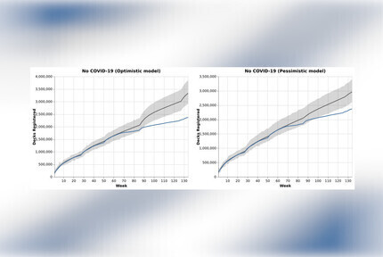
What if COVID-19 never happened ?
Now that we have a decent model at hand, we can get creative and model how many decks would have been registered in case
the pandemic never happened. To do this, we need to tweak the model a little. We’ll have to define covid_start as
pm.Data(), which can be altered after fitting the model. There also is a small change to the trace function to
get the sampling to work with this fixed parameter, init="adapt_diag" is added to avoid errors.
In the code below only changes from the previous are shown.
with pm.Model() as model_5:
    # ...
    # here we set the start of covid manually (based on previous notebook)
    # this way it can be changed after fitting the model
    covid_start = pm.Data("covid_start", 68)

    # ...

    # posterior
    trace_5 = pm.sample(1000, cores=10, chains=4, init="adapt_diag")
After fitting the model we can change the point where we want COVID-19 to start to a point in the future, using the
pm.sample_posterior_predictive() then will show the model, but without the effect of COVID-19.
with model_5:
    pm.set_data({"covid_start": 500})

chart_without_covid = plot_fit_altair(model_5, trace_5, model_data)
chart_without_covid
While this is great, it doesn’t offer much flexibility to change the model. Here for instance the interest in Mass Mutation and Dark Tidings might be overestimated as these were released during the pandemic. This might affect how and when people buy new decks. So it would be interesting if we could build a ‘Pessimistic’ model, where the interest in MM and DT is equal to the set with the least interest prior to the pandemic.
Once option here is to create a new model, where all priors are set to the posteriors from model_5. Then we can change
the values we want and run pm.sample_prior_predictive() to see how the model with our updated priors runs. In
the notebook you’ll find the optimistic version (with the exact parameters from model_5) and a pessimistic version
where the interest in MM and DT is set to the interest in WC, only the latter is shown here. While this does increase
the uncertainty on the predictions it comes with far more flexibility to play with the model.
Update 20/08/2021: In the GitHub repo you’ll find a better model which calculates the interest based on the pre-COVID rate
of registrations for all sets. This results in a far better prediction when using pm.Data to set the start of the
pandemic beyond the current time, which can be seen in this post.
The approach below still has merit in some cases, so I’ll leave it in, just know there is a better solution available
for this case.
with pm.Model() as model_7:
    # priors
    sigma = pm.Normal("sigma", mu=1.17, sigma=0.07)  # Sigma for likelihood function

    weekly_registrations = pm.Normal("weekly_registrations", mu=1.55, sigma=0.06)

    # Model extra registrations due to shifting interest (like new sets being released)
    # The interest factor is calculated on a weekly basis
    decay_factor = pm.Normal("decay_factor", mu=0.84, sigma=0.01)

    cota_interest = pm.Normal("cota_interest", mu=4.11, sigma=0.19)
    aoa_interest = pm.Normal("aoa_interest", mu=1.7, sigma=0.16)
    wc_interest = pm.Normal("wc_interest", mu=0.95, sigma=0.13)
    # Maybe people's buying behaviour responds differently to
    # the release of a new set during COVID.
    # Set the two most recent sets to a worst case scenario
    mm_interest = pm.Normal(
        "mm_interest", mu=0.95, sigma=0.13
    )
    dt_interest = pm.Normal(
        "dt_interest", mu=0.95, sigma=0.13
    )

    interest_decayed = [cota_interest]

    for i in range(len_observed - 1):
        new_element = interest_decayed[i] * decay_factor
        if i == 27:
            new_element += aoa_interest
        if i == 50:
            new_element += wc_interest
        if i == 85:
            new_element += mm_interest
        if i == 126:
            new_element += dt_interest
        interest_decayed.append(new_element)

    # there were 150k decks registered the first week, that is the initial value
    y0 = tt.zeros(len_observed)
    y0 = tt.set_subtensor(y0[0], 15)

    outputs, _ = theano.scan(
        fn=lambda t, y, intfac: tt.set_subtensor(
            y[t], (weekly_registrations * (1 + intfac[t])) + y[t - 1]
        ),
        sequences=[tt.arange(1, len_observed)],
        outputs_info=y0,
        non_sequences=[interest_decayed],
        n_steps=len_observed - 1,
    )

    total_registrations = pm.Deterministic("total_registrations", outputs[-1])

    # Likelihood
    likelihood = pm.Normal(
        "y", mu=total_registrations, sigma=sigma, observed=model_data.Total_scaled
    )
As you can see, in the pessimistic model the bumps caused by releasing the latest sets are far more modest and in line with previous releases. This could indicate that purchasing behaviour is different during COVID-19 (which I fully expect to be the case).
Conclusion
While probabilistic programming is somewhat different from regular programming, though PyMC3 makes this transition manageable! Creating these models however is far more involved than fitting a machine learning model, though this comes with advantages: These models are very easy to inspect and understand what each parameter is doing and, we can change parameters to model scenarios for which we don’t have any data. Unlike machine learning models which are often black boxes, with internals that are hard to understand and even harder to change, this is a huge advantage when predicting things.
The interpretation of some of these results in a non-technical way can be found here! Note that this is all about the number of registered decks, if you are interested in the total number of printed decks, have a look a this post.
Resources
In case you want to get started with PyMC3 yourself, here are the resources I’ve been using.
- PyMC3 Workshop from Thomas Wiecki which taught me a lot of tricks that were applied here
- The official PyMC3 documentation
- Bayesian Analysis with Python
- PyMC Developers channel on YouTube
Liked this post ? You can buy me a coffee