Minimalist Art Using a Genetic Algorithm
a different take on Vermeer's Girl with a Pearl Earring
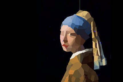
While the genetic algorithm in the previous post worked very well, it didn’t quite produce the style of minimalist artwork I was trying to achieve. Furthermore, it didn’t allow the chromosomes to evolve using duplication and deletion of existing genes (which is very common in biology). So after mulling over these issues a few days, I found a solution using a Voronoi diagram. The final result (shown below) is much closer to what I was aiming for. The painting to re-drawn by the algorithm this time is Vermeer’s Girl with a Pearl Earring.

Voronoi diagrams (aka partitions or cells)
The plot below illustrates Voronoi diagrams; each blue point is an input point, black edges and orange corners are calculated. Black edges are equidistant between two neighboring points and orange points (endpoints of an edge) are equidistant between three neighbors. This creates a polygon around each input point that is convex and non-overlapping. These polygons can be colored and drawn as solid shapes which creates a cell pattern. (You can find an entertaining explanation with more details here)
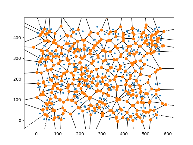
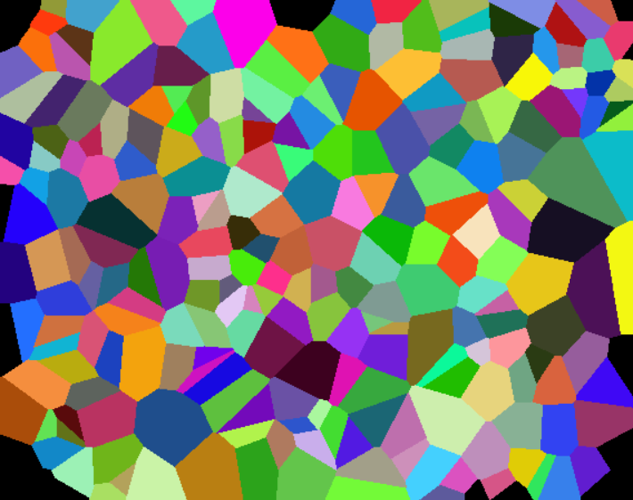
In Python Voronoi diagrams can easily be created and plotted from a list of points using the Voronoi class and voronoi_plot_2d
function which are included in SciPy. Excluding the imports you only need four lines of code !
from scipy.spatial import Voronoi, voronoi_plot_2d
import matplotlib.pyplot as plt
from random import randint

# Generate 200 random points between 0-500, 0-500
points = [(randint(0, 500), randint(0, 500)) for _ in range(200)]

vor = Voronoi(points)
voronoi_plot_2d(vor)
plt.show()
The new genes and chromosomes
Here the chromosome is a list of 2D points, each with an RGB color attached to it (the genes). These points can move, or the color can shift in a mutation step. The order of the points doesn’t matter and making a copy of a gene doesn’t have an impact on the image it produces. However it does provide additional ‘genetic material’ that can evolve and can create complexity as duplicate points start to diverge. Points can also be removed again from the chromosome, as Voronoi partitions are used, the gap will be filled automatically by the surrounding genes.
Here is the code for a single point, aka the gene. The code for the chromosome is nearly identical to that from the previous post with the exception of some trivial functions to duplicate genes and remove a random gene.
from random import shuffle, randint, choices, choice

class ColoredPoint:
    def __init__(self, img_width, img_height):
        self.coordinates = (randint(0, int(img_width)), randint(0, int(img_height)))
        self.color = (randint(0, 256),  # Random value for the Red channel
                      randint(0, 256),  # Random value for the Green channel
                      randint(0, 256),  # Random value for the Blue channel
                      255)              # The Alpha channel is fixed

    def mutate(self, sigma=1.0):
        mutations = ['shift', 'color']
        weights = [50, 50]

        mutation_type = choices(mutations, weights=weights, k=1)[0]

        if mutation_type == 'shift':
            self.coordinates = (self.coordinates[0] + int(randint(-10, 10)*sigma), self.coordinates[1] + int(randint(-10, 10)*sigma))
        elif mutation_type == 'color':
            red = self.color[0] + int(randint(-25, 25)*sigma)
            green = self.color[1] + int(randint(-25, 25)*sigma)
            blue = self.color[2] + int(randint(-25, 25)*sigma)

            self.color = (red, green, blue, 255)

            # Ensure color is within correct range
            self.color = tuple(
                min(max(c, 0), 255) for c in self.color
            )
Evolution through duplication
As points can be duplicated (and this initially has no impact on the image), this allows us to start with a relatively small number of points, evolve these for a while until we get close to the optimal. Then we can trigger a whole genome duplication where a chromosome is doubled. This will initially have no impact on the image, but as the duplicated points start to diverge, this can create additional complexity and a better fit to the target image. However, an excess of points will run rather slowly as it will take more time to draw the image (and since we are drawing hundreds of images each generation this matters) and it will be harder to randomly make a beneficial mutation. To solve this issue we need to reduce the number of genes every so often as well. (While I haven’t been able to test this, starting small, evolving to an optimum, duplicating the genome and evolving further should require fewer generations than when starting from a larger set of randomly initiated points.)
This is very similar to events that happened throughout the evolutionary history of many, many plants and animals, including humans !
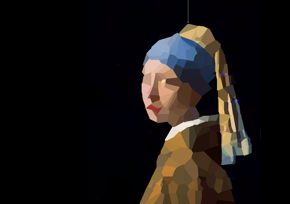
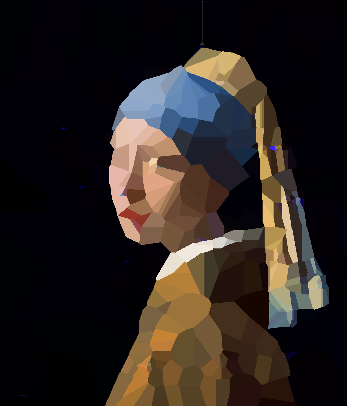
The strategy used to generate the image in the beginning of the post was to start with 250 points and evolve them for ~1000 generations, then double the number of points and evolve for another 1000 generations, shrink the genome by removing 100 points and double again. Then the population was left to evolve for a while and then force to shed 100 genes, this process was repeated a few times to end up with a final image that contains 600 points.
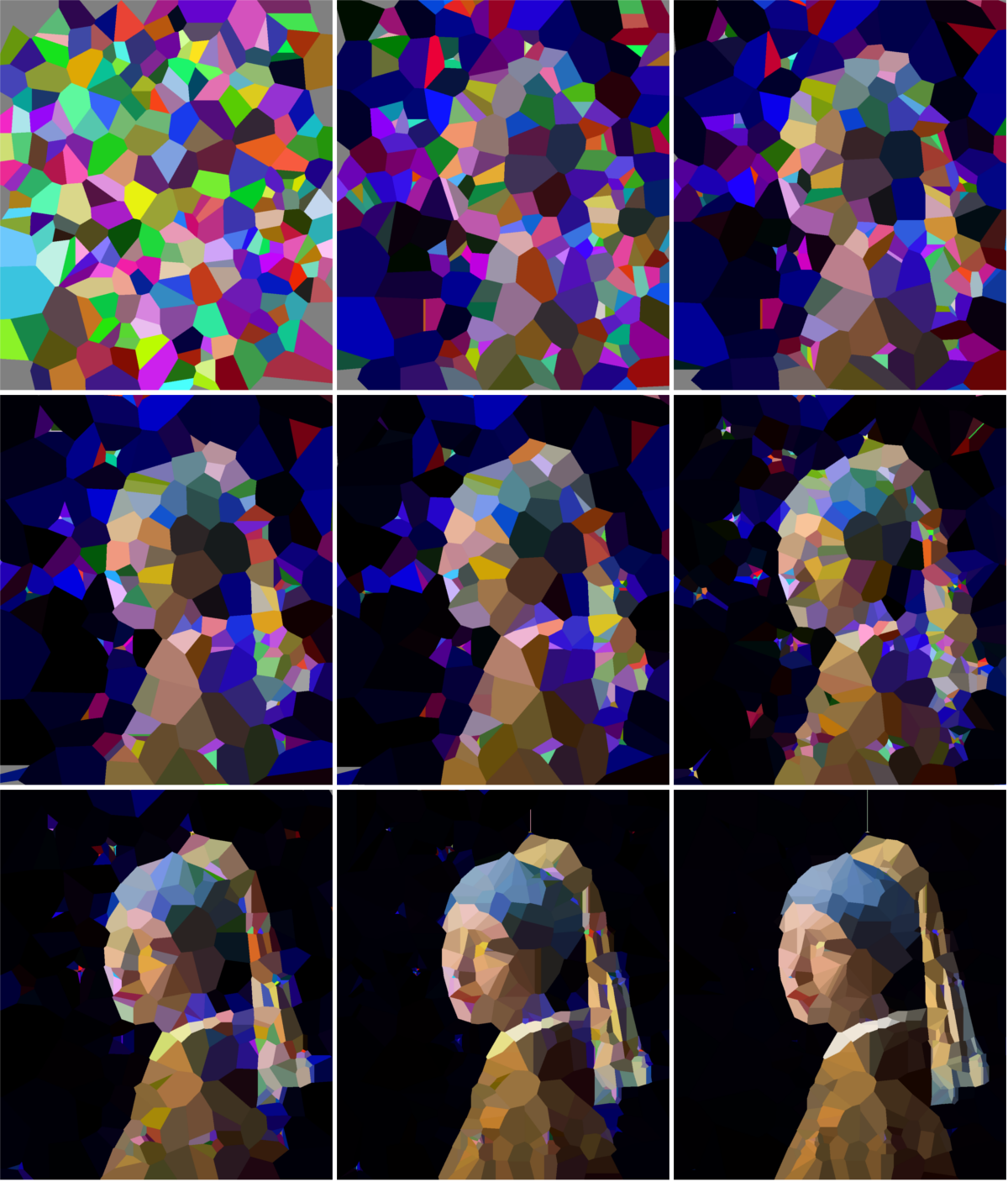
In the image above you can see the best individual (out of a population of 250) of generation 1, 250, 500, 750, 1000, 1500, 2500, 3500 and 5500. Between generation 1000-1500 and 2500-3500 there were duplications followed by a number of normal evolutionary steps and a few reductions steps. The complexity and detail of the image clearly increases at these steps.
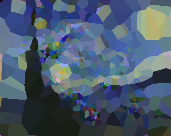
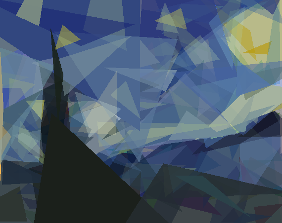
Comparison to the previous algorithm
I used this approach on Van Gogh’s A Starry Night as well, to compare the visual style of this algorithm with the previous one. Both images have a comparable fitness (distance to the target painting).
Conclusion
This approach generates a minimalist style I was initially aiming for, while allowing for duplication and loss events which mimic biology. Mission accomplished!
The code used here is mostly the same as the previous post, so I didn’t go over it in much depth. However, everything can be found on GitHub! Check the repository for the full working code.
Liked this post ? You can buy me a coffee